¶ Initial assessment of parameter variability (a priori distributions) with little site-specific information
¶ Contributors:
- Chair of Numerical Analysis (Technical University of Chemnitz): Chao Chang, Oliver Ernst, Moritz Poguntke
- Department Underground Space for Storage and Economic Use - Sub-department Rock Characterisation for Storage and Final Disposal (Federal Institute for Geosciences and Natural Resources): Werner Gräsle, Sibylle Mayr
- Chair of Soil Mechanics and Foundation Engineering (Technical University of Bergakademie Freiberg): Aqeel Afzal Chaudhry, Thomas Nagel
¶ Origin of parameter uncertainties
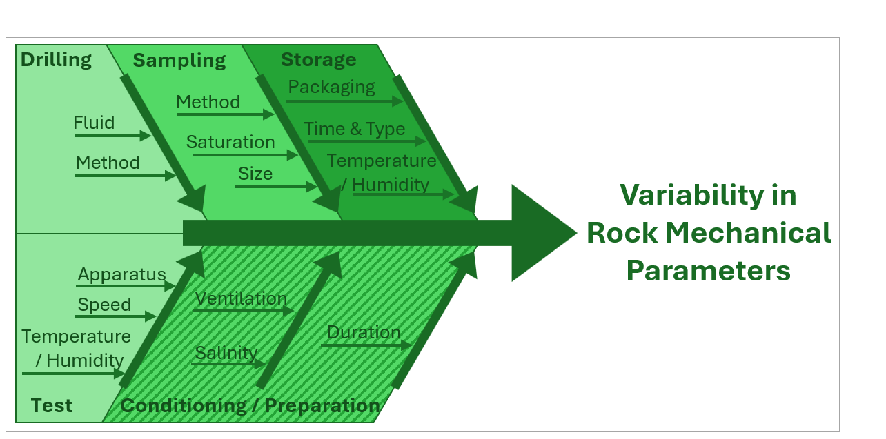
Modeling real-world phenomena, such as thermal, hydraulic, and mechanical (THM) interactions, involves the complex task of accurately representing systems while accounting for uncertainties in essential parameters. These uncertainties often stem from a range of data inaccuracies influenced by measurement limitations, environmental variability, and the inherent heterogeneity of samples, particularly in geologic contexts. Taking some examples from the figure on the side for instance, sensor accuracy, sample composition, conservation practices, and varying environmental conditions (e.g., temperature fluctuations) all contribute to the challenges of capturing reliable data. Addressing these factors is critical for creating models that can realistically reflect the behavior and interactions within natural systems, especially in fields reliant on precise simulation and forecasting.
The following examples demonstrate how variability/uncertainty in material properties affects model accuracy and reliability:
¶ Example 1: Shear strength
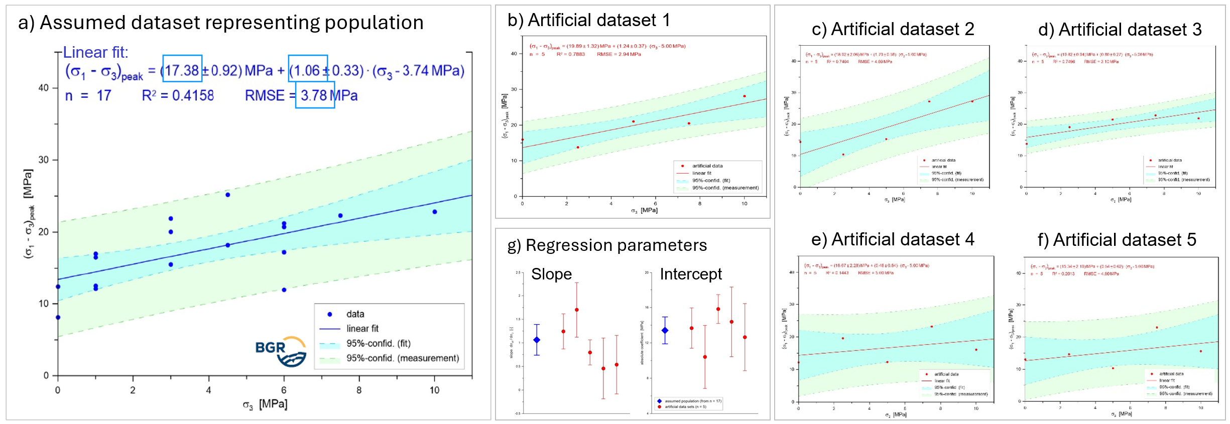
Shear strength is a critical parameter in geomechanical modelling that can be determined e.g. from cohesion (C) and angle of internal friction (phi). Sparse sampling (Diagram b-f. illustrating 5 data points for 5 artificial datasets, based on real measured data in Diagram a) for Oplalinus Clay with 17 data points) can have severe impact on the reliability of linear regression results with significant uncertainty in slope and intercept values (Diagram g).
¶ Example 2: Porosity
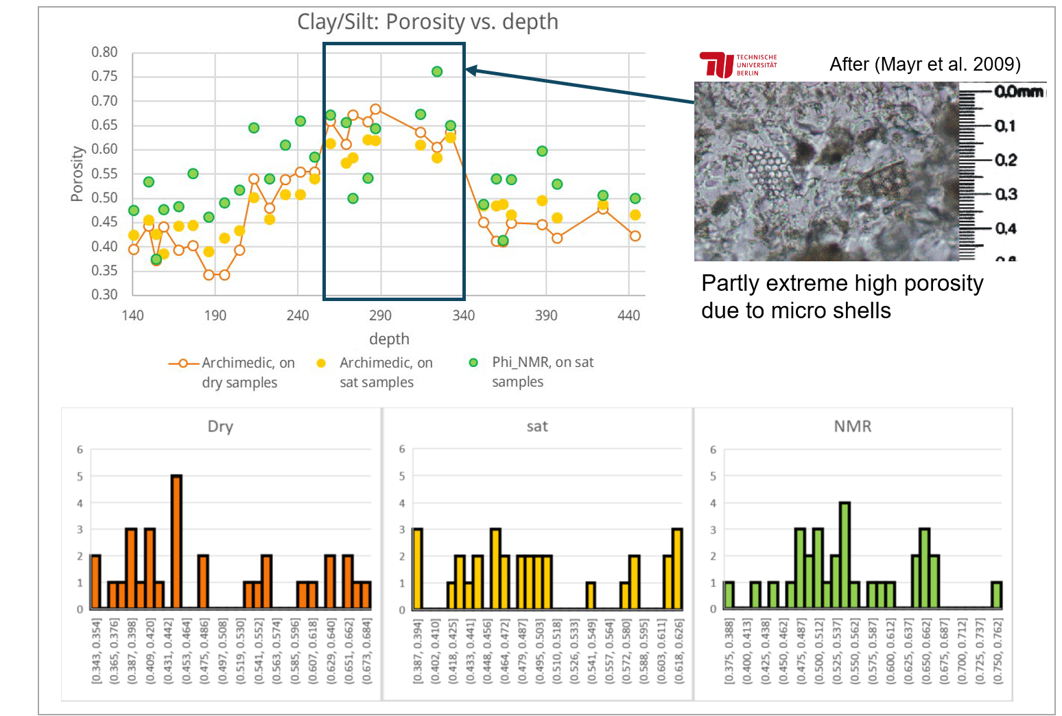
Porosity can be measured with various technique e.g. dry sample or saturated sample measurements, nuclear magnetic resonance (NMR) measurement. These techniques differ not in the manner of sample preparation but even in the state the sample is during measurement (such as dry vs. saturated state) which can lead to significantly different measured values (see Figure on the right):
- Measurements performed on dry samples generally resulted in higher data scatter compared to saturated samples;
- Porosity determined through NMR tended to be higher, possibly due to the presence of bound water that cannot be removed through drying.
Additionally, sample composition also plays a major role on the data scatter: in the example presented here, carbonate presence in the middle region causes extreme posotiy values during the mearuement due to micro-shell inclusions. This further complicates statistical analysis and model integration as it often can lead to non-Gaussion distribution.
¶ Parameter variability in THM models
To assess the geological integrity of the host rock, that essentially acts as a barrier in the final disposal of nuclear waste, understanding and predicting the behavior of the repository over a long period of time is critical. Numerical investigations of barrier integrity involves assigning material properties to the host rock for THM simulations. If complete information were available, the material properties would be known functions of location, and features such as inhomogeneity and anisotropy could be expressed by spatially varying tensor-valued coefficients. In reality, however, information about variations in the structure and properties of the geological barrier is incomplete, which brings forth the questions:
- At what scale must heterogeneity be accounted for?
- Are homogeneous models with random parametrization suitable to capture these parameter variations?
¶ Methodology
A common approach to analyze the impact of heterogeneity is to model the rock mass as homogeneous in sections (e.g. geological layers), and in each of these sections, the considered material parameter values are modelled as random variables. This modelling approach yields fully correlated parameter description at two neighboring locations. A universal tool to describe randomness with a more general structure is the utilization of random fields whose realizations are functions of space that are generally not constants - e.g. Gaussian random field determined by its mean value and its two-point correlation function. In this representation, anisotropy can occur in two forms:
- Statistical anisotropy: anisotropy present in the statistical covariance structure, leading to different correlation lengths along the principal axes of the random field;
- Physical anisotropy: anisotrpy associated with thermal/hydraulic/mechanical properties themselves, leading to random fields whose realisations are anisotropic tensor fields.
We present here a comparison study for both cases by choosing different correlation lengths for parallel and perpendicular directions for the first case and describing the dominant material property for each process in THM simulations as a tensor-valued random field for the second case: thermal conductivity for the thermal part, intrinsic permeability for the hydraulic part and elastic stiffness for the mechanical part. These properties play a key role in the evaluation of thermally induced excess pore water pressures and stress changes (Buchwald et. al., 2020; Chaudhry et. al., 2021).
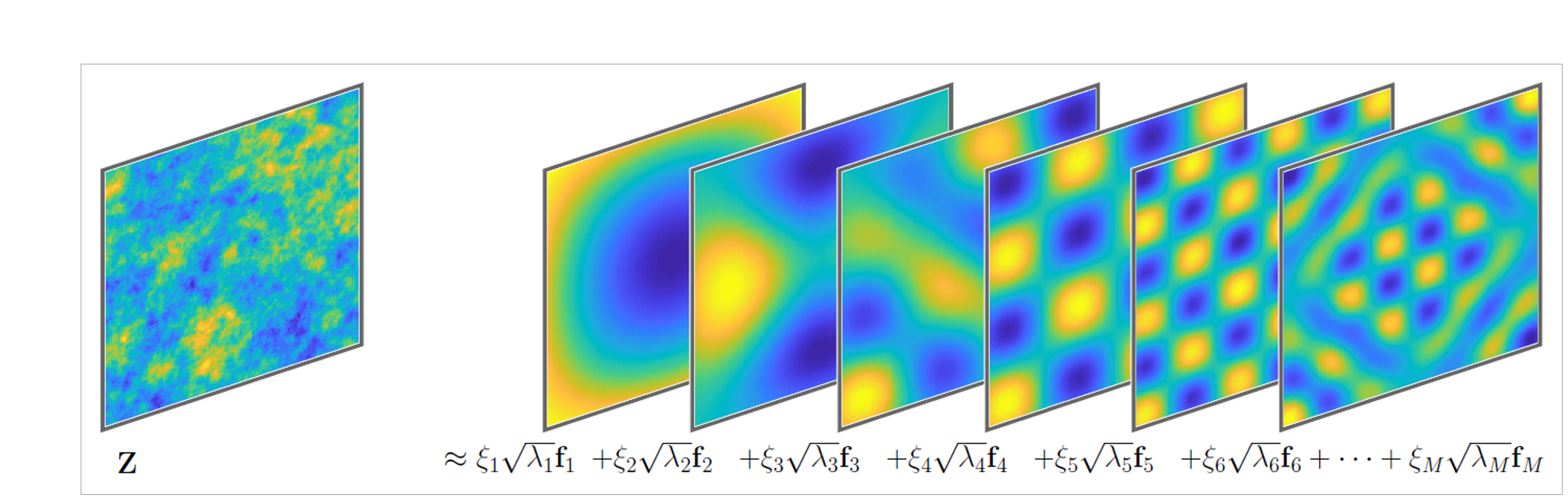
To generate the random fields, we use the Karhunen-Loève expansion, which decomposes a random field into a series of orthogonal modes: the eigenfunctions capture the variability of the field at different spatial scales, while the associated eigenvalues quantify the proportion of variance carried by these eigenfunctions. The formula used to describe realizations for Gaussian random fields is given as:
$${Z(x,\xi) = Z_{mean}(x) + \sum^M_{i=1}(\xi_i \sqrt{\lambda_i} f_i(x)) }$$
where Zmean(x) is the mean of the field ξi ~ N(0,1), and fi and λi are eigenfunctions and eigenvalues of the covariance operator respectively, computed by solving the generalized eigenvalue problem numerically:
$${C f_i = \lambda_i M f_i}$$
$${ [C]_{i,j} = \int_D \phi_j(x) \int_D c(x,y) \phi_j(y) dy dx}$$
where φ is basis function, and c(x,y) is kernel/covariance function.
Solving the above problem for THM simulations brings in challenges:
- The covariance matrix [C]i,j involves integration of non-smooth covariance functions c(x,y).
- The covariance matrix [C]i,j is dense of size N x N for N degree of freedoms, which leads to expensive computational storage and matrix-vector product calculations.
- The above problem requires eigen-solver.
We tackle these challenges by taking the following steps:
- To alleviate the singularity issue, we use the Sauter-Schwab quadrate scheme (Sauter and Schwab 2011).
- To lower the computational efforts needed to solve the problem, we introduce hierarchical matric approximation for the covariance matrix, which effectively reduces matrix assembly and matrix-vector multiplication from O(N2) to O(N logN).
- We implement the Thick-restart Lanczos eigen solver (Wu and Simon 2000).
¶ Impact of inhomogeneity and anisotropy
The case study used for the anisotropy and inhomogeneity impacts is a benchmark-type setup from previous cases (Chaudhry et al. 2021, Buchwald et al. 2020, Pitz et al. 2023): a circular 2D domain of 100m diameter with a circular hole in the center representing the emplaced high-radioactive waste cell (diameter of 2.48m).
We identify 3 input parameters with high degree of uncertainty: thermal conductivity (λ), intrinsic permeability (k) and Young’s modulus (E). To assess the impact of inhomogeneity and anisotropy, these three parameters are defined to represent said behavior. For clarity, we distinguish between material and statistical anisotropy:
- Material anisotropy: refers to the intrinsic, direction-dependent behavior of a material’s physical property. E.g., intrinsic permeability may vary depending on the orientation (parallel vs. perpendicular to bedding plane in the rock). It is modeled using tensor-valued random fields where the random realization represents symmetric positive-definite matrices aligned with specific principal directions.
- Statistical anisotropy: describes anisotropy in the correlation structure of random fields representing the material property, meaning that the spatial variability of properties depends on direction, resulting in different correlation lengths along principal axes (e.g., longer correlation along the bedding plane than perpendicular to it). It is modelled by modifying the covariance function to include anisotropic scaling factors that define how variability stretches differently in each direction.
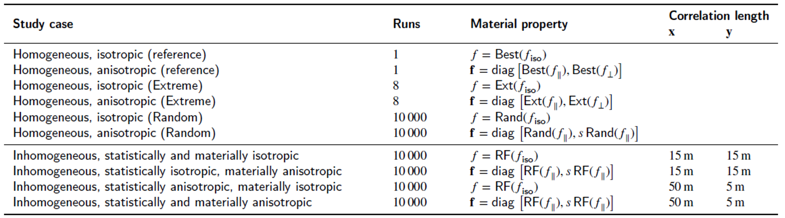
A list of established scenarios is provided in the table below. In the first six homogeneous cases, spatially constant values were used for the three uncertain inputs. In the two cases labeled “Extreme”, all eight combinations of the three extreme values Ext ∈ {Min, Max} were simulated. In the cases labeled “Random,” the spatially constant values of the three inputs were randomly sampled from their probability distributions. The last four cases employed (spatially varying) random fields for the three input quantities.
As several cases were designed in this study to isolate the effects for both inhomogeneity and anisotropy, the detailes for each cases are discussed in parallel to emphasize the impacts. A brief summary of the most relevant results are listed below. For more details the reader is kindly referred to the article from Chaudhry et al. 2025.
¶ Homogeneous cases
- Isotropic vs. Anisotropic results: For isotropic cases, results exhibit radial symmetry in temperature, fluid pressure, displacement, and stress contours. Anisotropic cases show elliptical contours for output variables, with major axes depending on the dominant material direction. This reversal of axes at different radii is attributed to complex coupling effects.
- Extreme cases: Thermal conductivity predominantly influences temperature. Other parameters (permeability, Young’s modulus) show secondary effects driven by coupling mechanisms. Pressure and displacement exhibit complex interactions, with extreme combinations of parameters producing localized peaks and deviations in response variables.
- Random cases: Variability in output variables is tighter for random cases (95% bounds) compared to extreme cases, except for temperature, which depends more linearly on thermal conductivity.Coupled input-output relationships lead to variations in output bounds not captured by simplistic random sampling.
¶ Inhomogeneous cases
- Statistically and Materially Isotropic: Incorporating random fields adds spatial variability, producing smoother transitions in temperature, pressure, and displacement fields. Compared to homogeneous models, inhomogeneity reduces sharp peaks in stress responses, reflecting the averaging effect of spatial randomness.
- Statistical Anisotropy: Anisotropic correlation lengths (e.g., 50 m in x-direction vs. 5 m in y-direction) result in elongated or compressed response fields. Stress indicators show anisotropy-induced asymmetries in von Mises stress and effective hydrostatic pressure.
- Material Anisotropy: Variability in material properties (e.g., anisotropic permeability and thermal conductivity) introduces stronger directional effects in fluid flow and stress fields. Observed differences confirm the need for material anisotropy in predictive models to capture shear and tensile failure risks effectively.
- Combined Anisotropy and Inhomogeneity: Statistical and material anisotropies combined with random fields yield the most realistic outputs. Results align well with expected behavior in complex geological media, reflecting the interplay of spatial variability and directional material responses.
¶ References
- D. Jaeggi, P. Bossart, L. Wymann (2014). Kompilation der lithologischen Variabilität und Eigenschaften des Opalinus-Ton im Felslabor Mont Terri. Expertenbericht im Rahmen der Beurteilung des Vorschlags von mindestens zwei geologischen Standortgebieten pro Lagertyp, Etappe 2, Sachplan geologische Tiefenlager.
- A. A. Chaudhry, C. Zhang, O. G. Ernst, T. Nagel (2025). Effects of inhomogeneity and statistical and material anisotropy on THM simulations. Reliability Engineering and System Safety, 260. DOI:10.1016/j.ress.2025.110921